
A new technology to store 650 MByte of data on a CD had been developed based on the same basic principles used by the telco industry for their optical fibres, but the way it had been implemented had brought the price down to levels that industry could only dream of. Storing that impressive amount of data on a 12-cm physical carrier was a done deal, but transmitting the same data over a telephone line, would take a long time, because the telephone network had been designed to carry telephone signals with a nominal bandwidth of just 4 kHz.
So, the existing telephone network was unsuitable for the future digital world, but what should be an evolutionary path to a network handling digital signals? Two schools of thought formed, the visionaries and the realists. The first school aimed at replacing the existing network with a brand new optical network, capable of carrying hundreds – maybe more – Mbit/s per fibre. This was technically possible and had already been demonstrated in the laboratories, but the issue was bringing the cost of that technology to acceptable levels, as the CE industry had done with the CD. The approach of the second school was based on more sophisticated considerations (this does not imply that the technology of optical fibres is not sophisticated): if the signals converted to digital form are indeed bandwidth-limited, as they have to be if the Nyquist theorem is to be applied, contiguous samples are unlikely to be radically different from one another. If the correlation between contiguous samples can be exploited, it should be possible to reduce the number of bits needed to represent the signals without affecting its quality.
Both approaches required investments in technology, but of a very different type. The former required investing in basic material technology, whose development costs had to be borne by suppliers and the deployment costs by the telcos (actually, because of the scarce propensity of manufacturers to invest on their own, telcos would have to fund that research as well). The latter required investing in algorithms to reduce the bitrate of digital Audio and Video (AV) signals and devices capable of performing what was expected to be a very high number of computations per second. In the latter case it could be expected that the investment cost could be shared with other industries. Of course either strategy, if lucidly implemented, could have led the telco industry to world domination, given the growing and assured flow of revenues that the companies providing the telephone service enjoyed at that time. But you can hardly expect such a vision from an industry accustomed to cosset Public Authorities to preserve its monopoly. These two schools of thought have dominated the strategy landscape of the telco industry, the former having more the ears of the infrastructure portion of the telcos and the latter having more the ears of the service portion.
The first practical application of the second school of thought was the facsimile. The archaic Group 1 and Group 2 analogue facsimile machines required 6 and 3 minutes, respectively, to transmit an A4 page. Group 3 is digital and designed to transmit an A4 page scanned with a density of 200 Dots Per Inch (DPI) with a standard number of 1728 samples/scanning line and a number of scanning lines of about 2,300 if the same scanning density is used vertically (most facsimile terminals, however, are set to operate at a vertical scanning density of ½ the horizontal scanning density).
Therefore, if 1 bit is used to represent the intensity (black or white) of a dot, about 4 Mbits are required to represent an A4 page. It would take some 400 seconds to transmit this amount of data using a 9.6 kbit/s modem (a typical value at the time Group 3 facsimile was introduced), but this time can be reduced by a factor of about 8 (the exact reduction factor depends on the specific content of the page) using a simple but effective scheme based on the use of:
- “Run lengths” of black and white samples: instead of sample values
- Different code words to represent black and white run lengths: their statistical distribution is not uniform (e.g. black run lengths are more likely to be shorter than white ones). This technique is called Variable Length Coding (VLC).
- Different VLC tables for black and white run lengths: black and white samples on a piece of paper have different statistics.
- Information of the previous scan line: if there is a black dot on a line, it is more likely that there will be a black dot on the same vertical line one horizontal scanning line below than if there had been a white dot.
Group 3 facsmile has been the first great example of successful use of digital technologies in the telco terminal equipment market.
But let’s go back to speech, the telco industry’s bread and butter. In the early years, 64 kbit/s for a digitised telephone channel was a very high bitrate in the local access line, but not so much in the long distance, where bandwidth, even without optical fibres, was already plentiful. Therefore, if speech should ever reach the telephone subscriber in digital digital form, a lower bitrate had to be achieved.
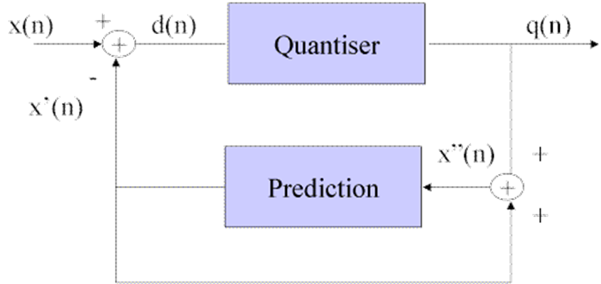
The so-called Differential PCM Pulse Code Modulation (DPCM) was widely considered in the 1970s and ’80s because the technique was simple and offered a moderate compression. DPCM was based on the consideration that, since the signal has a limited bandwidth, consecutive samples will not be so different from one another, and sending the VLC of the difference of the two samples will statistically require fewer bits. In practice, however, instead of subtracting the previous sample from the actual sample, it is more effective to subtract an estimate of the previous sample, as shown in the figure below. Indeed, it is possible to make quite accurate estimates because speech has some well identified statistical characteristics given by the structure of the human auditory system. Taking into account the sensitivity of the human ear, it is convenient to quantise the difference finely if the difference value is small and more coarsely if the value is larger before applying VLC coding. The decoder is very simple as the output is the running sum of each differential sample and the value of reconstructed samples filtered through the predictor.
 |
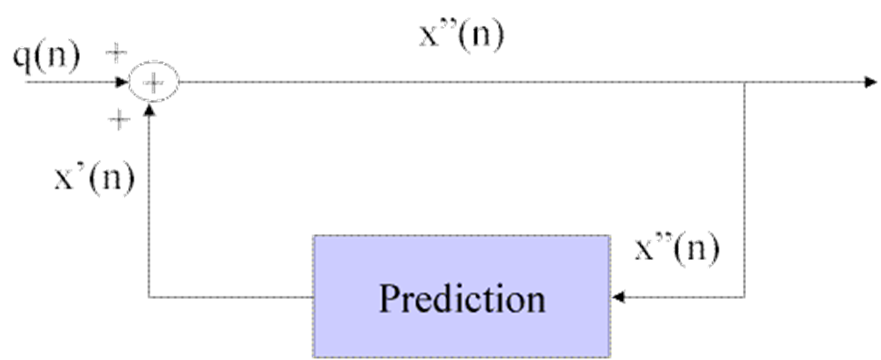 |
Figure 1 – DPCM encoder and decoder
DPCM was a candidate for video compression as well but the typical compression ratio of 8:3 deemed feasible with DPCM was generally considered inadequate for the high bitrate of digital video signals. Indeed, using DPCM one could hope to reduce the 216 Mbit/s of a digital television signal down to about 70 Mbit/s, a magic number for European broadcasters because it was about 2 times 34 Mbit/s, an element of the European digital transmission hierarchy. For some time this bitrate was fashionable in the European telecom domain because it combined the two strategic approaches: DPCM running at a clock speed of 13.5 MHz was a technology within reach of the early 1980s and 70 Mbit/s was “sufficiently high” to still justify the deployment of optical fibres to subscribers.
To picture the atmosphere of those years, let me recount the case when Basilio Catania, then Director General of CSELT and himself a passionate promoter of optical networks, opened a management meeting by stating that because 210 Mbit/s was going to be feasible as subscriber access soon (he was being optimistic, it is becoming, if not economically, at least strategically feasible even now, 35 years later), and because 3 television programs was what a normal family would need, video had to be coded at 70 Mbit/s. The response to my naïve question if the solution just presented was the doctor’s prescription, was that I was no longer invited to the follow-up meetings. Needless to say that the project of bringing 3 TV channels to subscribers went nowhere.
Another method, used in music coding, subdivides the signal bandwidth in a number of subbands, each of which is quantised with more or less accuracy depending on the sensitivity of the ear to the particular frequency band. For obvious reasons this coding method is called Subband Coding (SBC).
Yet another method uses the properties of certain linear transformations. A block of N samples can be represented as a point in an N-dimensional space and a linear transformation can be seen as a rotation of axes. In principle each sample can take any value within the selected quantisation range, but because samples are correlated, these will tend to cluster around a hyper-ellipsoid in the N-dimensional space. If the axes are rotated, i.e. an “orthogonal” linear transformation is applied, each block of samples will be represented by different numbers, called “transform coefficients”. In general, the first coordinate will have a large variance, because it corresponds to the axis of the ellipsoid that is most elongated, while the subsequent coordinates will tend to have lesser variance.
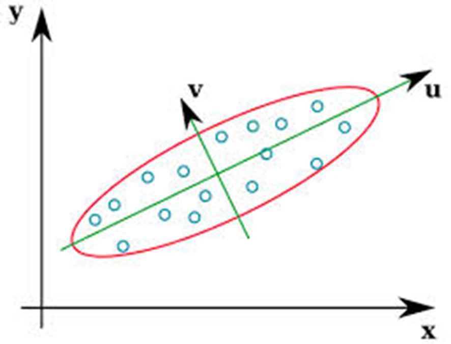
Figure 2 – Axis rotation in linear transformation
If the higher-variance transformed coefficients (the u axis in the figure) are represented with higher accuracy and lower-variance coefficients are represented with lower accuracy, or even discarded, a considerable bit saving can be achieved, without affecting the values of the samples too much when the original samples are reproduced approximately, using available information, by applying an inverse transformation.
The other advantage of transform coding, besides compression, is the higher degree of control of the number of bits used that can be obtained compared with DPCM. If the number of samples is N and one needs a variable bitrate scheme between, say, 2 and 3 bits/sample, one can flexibly assign the bit payload between 2N and 3N.
A major shortcoming of this method is that, in the selected example, one needs about NxN multiplications and additions. The large number of operations is compensated by a rather simple add-multiply logic. “Fast algorithms” need a smaller number of multiplications (about Nxlog2(N)), but require a considerable amount of logic driving the computations. An additional concern is the delay intrinsic in transform coding. By smartly programming the instructions, this roughly corresponds to the time it takes to build the block of samples. If the signal is, say, music sampled at 48 kHz, and N=1,024, the delay is about 20 ms, definitely not a desirable feature for real-time communication, of some concern in the case of real-time broadcasting and of virtually no concern for playback from a storage device.
The analysis above applies particularly to a one-dimensional signal like audio. Pictures, however, present a different challenge. In principle the same algorithms as used in the one-dimensional (1D) audio signal could be applied to pictures. However, transform coding of long blocks of 1D picture samples (called pixel, from picture element) was not the way to go because image signals have a correlation that dies out rather quickly, unlike audio signals that are largely oscillatory in nature and whose frequency spectrum can then be analysed using a large number of samples. Applying linear transformations to 2D blocks of samples was very effective, but this required storing at least 8 or 16 scanning lines (the typical block size choices) of 720 samples each (the standard number of samples of a standard television signal), a very costly requirement in the early times (second half of the 1970s) when the arrival of the 64 Kbit RAM chip after the 16 Kbit Random Access Memory (RAM) chip, although much delayed, was hailed as a great technology advancement (today we have 128 Gbyte RAM chips) .
Eventually, the Discrete Cosine Transform (DCT) became the linear transformation of choice for both still and moving pictures. It is therefore a source of pride for myself that my group at CSELT has been one of the first to investigate the potential of linear transforms for picture coding, and probably the first to do so in Europe on a non-episodic fashion. In 1979 my group implemented one of the first real-time still-picture transmission systems that used DCT and exploited the flexibility of transform coding by allowing the user to choose between transmitting more pictures per unit of time at a lesser quality or fewer pictures at a higher quality.
Pictures offered another dimension compared to audio. Correlation within a picture (intra-frame) was important, but much more could be expected by exploiting inter-picture (inter-frame) correlation. One of the first algorithms considered was called Conditional Replenishment (CR) coding. In this system a frame memory contains the previously coded frame. The samples of the current frame are compared line by line, using an appropriate algorithm, with those of the preceding frame. Only the samples considered to be “sufficiently different” from the corresponding samples of the previously coded frames are compressed using intra-frame DPCM and placed in a transmission buffer. Depending on the degree of buffer fullness, the threshold of “change detection” can be raised or lowered to produce more or fewer bits.
A more sophisticated algorithm is so-called Motion Compensation (MC) video coding. In its block-based implementation, the encoder looks for the best match between a given block of samples of the current frame and a block of samples of the preceding frame. For practical reasons the search is performed only within a window of reduced size. Then the differences between the given block and the “motion-compensated” block of samples are encoded using again a linear transformation. From this explanation it is clear that inter-frame coding requires the storage of a full frame, i.e. 810 Kbyte for a digital television picture of 625 lines. When the cost of RAM decreased sufficiently, it became possible to promote digital video as a concrete proposition for video distribution.
From the 1960s a considerable amount of research was carried out on compression of different types of signals: speech, facsimile, videoconference, music, television. The papers produced at conferences or academic journals can be counted by hundreds of thousand and the filed patents by the tens of thousands. Several conferences developed to cater to this ever-increasing compression coding research community. At the international level, the International Conference on Acoustics, Speech and Signal Processing (ICASSP), the Picture Coding Symposium (PCS) and the more recent International Conference on Image Processing (ICIP) can be mentioned. Many more conferences exist today on special topics or at the regional/national level. Several academic journals dealing with coding of audio and video also exist. In 1988 I started “Image Communication”, a journal of the European Signal Processing Association (EURASIP). During my tenure as Editor-in-Chief of that journal until 1999, more than 1,000 papers were submitted for review to that journal alone.
I would like to add a few words about the role that CSELT and my lab in particular had in this space. Already in 1975 my group had received the funds to build a simulation system that had A/D and D/A converters for black and white and PAL television, a solid state memory of 1 Mbyte built with 4 kbit RAM chips, connected to a 16-bit minicomputer equipped with a Magnetic Tape Unit (MTU) to move the digital video data to and from the CSELT mainframe where simulation programs could be run.
In the late 1970s the Ampex digital video tape recorder promised to offer the possibility to store an hour of digital video. This turned out not to be possible because the input/output of that video tape recorder was still analogue. With the availability of the 16 kbit RAM chips we could build a new system called Digital Image Processing System (DIPS) that boasted a PDP 11/60 with 256 Kbyte RAM interfaced to the Ampex digital video tape recorder and a 16 Mbyte RAM for real-time digital video input/output.

Fig. 3 – The DIPS Image Processing System
But things had started to move fast and my lab succeeded in building a new simulation facility called LISA by securing the latest hardware: a VAX 780 interfaced to a system made of two Ampex disk drives capable of real-time input/output of digital video according to ITU-R Recommendation 656 and, later, a D1 digital tape recorder.
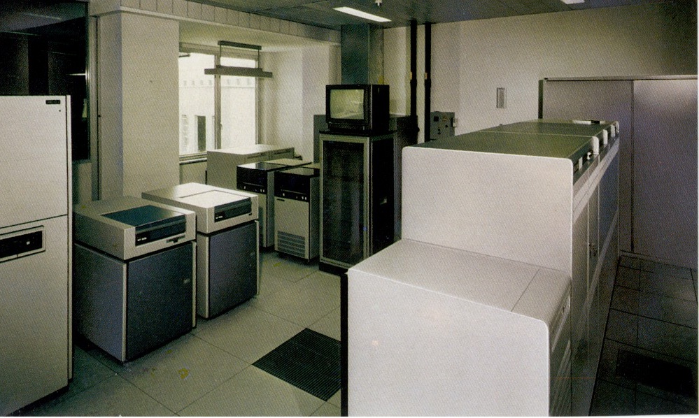
Fig. 4 The LISA Image Processing System